Brief Introduction
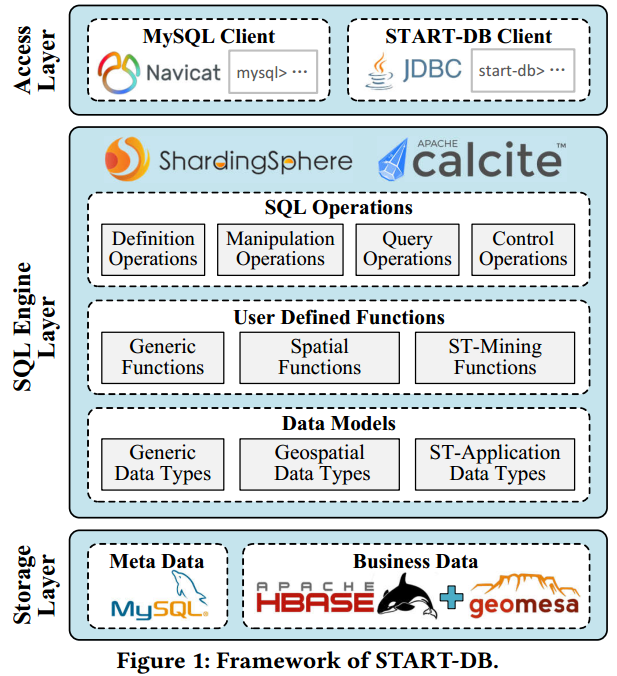
START-DB is an open-source spatio-temporal data management and mining system. It helps users to manage and mine large-scale spatio-temporal data conveniently. START-DB consists of three layers: Storage Layer, SQL Engine Layer and Access Layer. In Storage Layer, the spatio-temporal data is stored in HBase and indexed with GeoMesa, and the meta data is stored in MySQL. The SQL Engine Layer is implemented based on Apache Calcite and Apache ShardingSphere. We preset many spatio-temporal data types and mining operations in the SQL engine. In Access Layer, as START-DB is compatible with MySQL protocol, existing MySQL clients can connect to START-DB directly.
Key Features
(1) Scalable
START-DB stores the spatio-temporal data in a distributed NoSQL store, i.e., HBase, thus can support big data storage.
(2) Holistic
It supports not only CRUD (i.e., create, read, update, delete) operations, but also many spatio-temporal data mining operations, such as shortest path and trajectory map-matching.
(3) User-Friendly
It implements a complete SQL engine based on Apache Calcite, and incorporates a powerful database middleware Apache ShardingSphere. As a result, any operation can be achieved by a standard SQL statement.
Github Source Code
Prerequisites
1. Install docker and docker-compose in your computer: https://docs.docker.com/compose/install/
2. Install JDK 1.8 in your computer: https://www.oracle.com/fr/java/technologies/javase/javase8-archive-downloads.html
3. Check both docker and JDK have been added to your system environmental variable. If you system is output as follows, it indicates that your system is OK.
Demonstration Tutorials
Here is the screen recording of our demonstraion.
Now, let's experience START-DB by executing the following statements one by one.
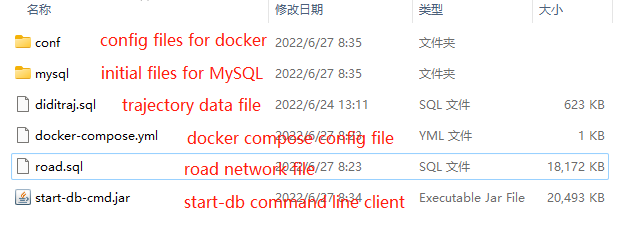
1. Download Necessary Files
Download the zip file SIGSPATIAL-Demo.zip, and extract it in your computer. The files are as follows:
2. Launch the Services
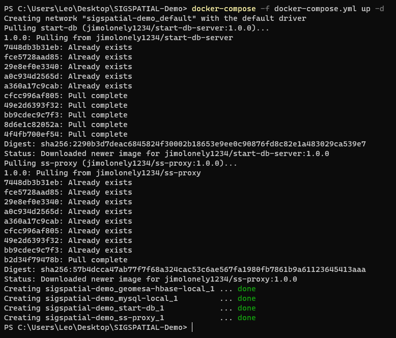
Enter folder SIGSPATIAL-Demo, open a command line client of Window system, and input the following command:
docker-compose -f docker-compose.yml up -d
The screen shot is shown as follows:
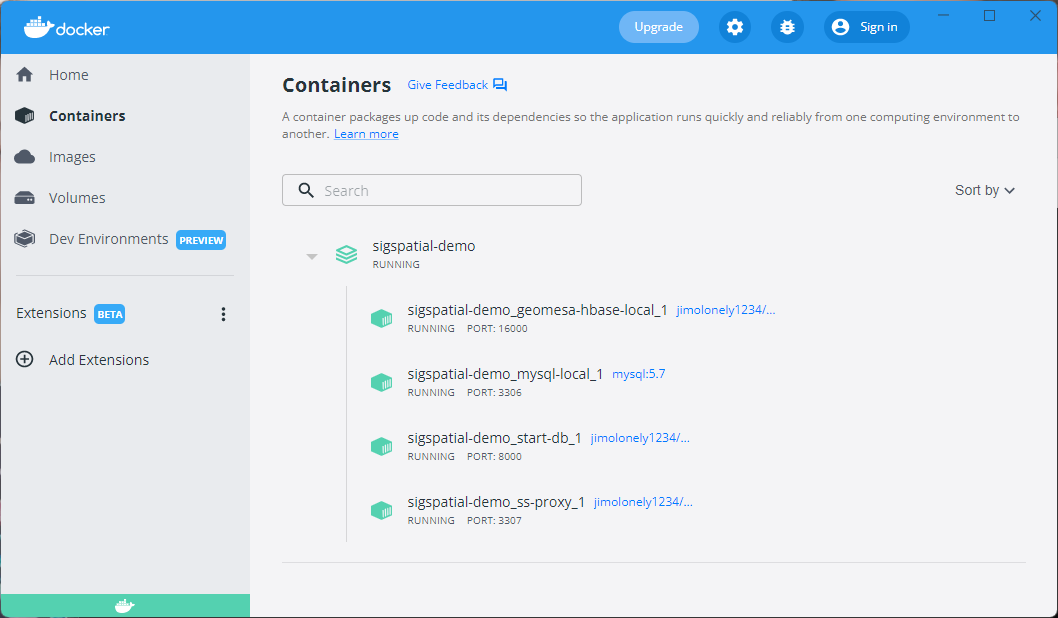
We can also see the service containers in the Docker Desktop:
3. Connect to Services
Input the following command to connect to the START-DB service:
java -jar start-db-cmd.jar -u root -p start-db
where
root is the inbuilt user, and start-db is the password. The screen shot is shown as follows. We can also see that for each user, we preset a default database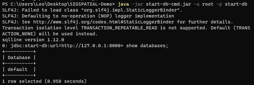
4. Create Database
Create a database
sigspatialdemo.
create database sigspatialdemo;
Set the database
sigspatialdemo as default.
use sigspatialdemo;
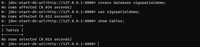
5. Create Tables
Create a table
diditraj that contains two fields tid, traj.
create table diditraj (tid string, traj trajectory);
Create a table
road that contains two fields rsid, rs.
create table road (rsid integer, rs roadsegment);

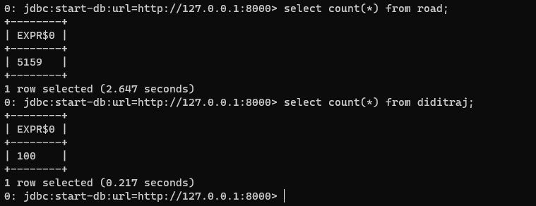
6. Load data into the tables
Load data to table
diditraj. Here diditraj.sql is the SQL file defining DML statements that insert trajectory data into table diditraj.
!source diditraj.sql
Load data to table
road.
!source road.sql
Note currently,
source command is executed in the client-side, so it must be prefixed with !. Also, this command should not end with ;.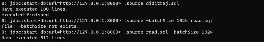
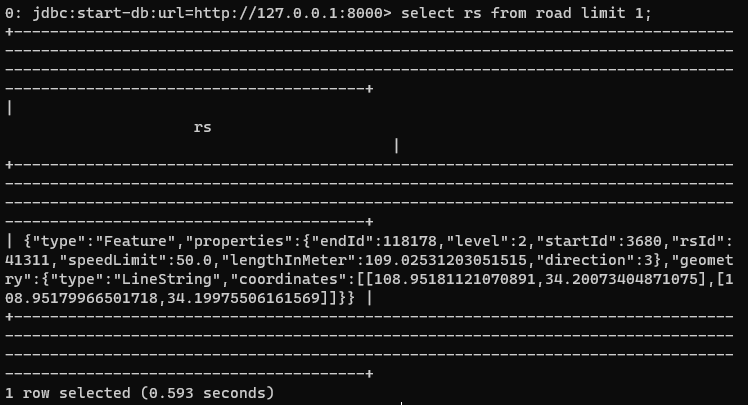
7. Select Data
We can query the data by the following statement. For
trajectory and roadsetment data types, we display it with GeoJSON format, thus we can visualize them is any standard GEO visualization tool such as QGIS and http://geojson.io/.
select rs from road limit 1;
8. Shortest Path
Perform a shortest path query with the following statement. Here,
st_rn_makeRoadNetwork is a user defined function (UDF) that creates a road network, and st_makePoint is another UDF that makes a Point object.
SELECT st_rn_shortestPath(st_rn_makeRoadNetwork(collect_list(rs)), st_makePoint(108.96978378295897,34.218828781354915), st_makePoint(108.99587631225586,34.23571867070669)) FROM road;
The result of this query is shown in GeoJSON format, thus we can view the result in any standard GEO visualization tool such as QGIS and http://geojson.io/. The following picture shows that we copy the result to http://geojson.io/, and the path is as the black line.
9. Map Match
Given a GPS trajectory, we can perform a map-matching operation with the following SQL statement. Here,st_traj_fromGeoJSON is a UDF that make a trajectory from a GeoJSON string.
SELECT st_traj_mapMatch(st_rn_makeRoadNetwork(collect_list(rs)), st_traj_fromGeoJSON('{"type":"FeatureCollection","features":[{"type":"Feature","properties":{"time":"2018-10-09 07:35:17.0"},"geometry":{"type":"Point","coordinates":[109.00295444870362,34.238112453328014]}},{"type":"Feature","properties":{"time":"2018-10-09 07:35:20.0"},"geometry":{"type":"Point","coordinates":[109.00296440590697,34.23811242319842]}},{"type":"Feature","properties":{"time":"2018-10-09 07:35:23.0"},"geometry":{"type":"Point","coordinates":[109.00295444870362,34.238112453328014]}},{"type":"Feature","properties":{"time":"2018-10-09 07:35:27.0"},"geometry":{"type":"Point","coordinates":[109.00295444870362,34.238112453328014]}},{"type":"Feature","properties":{"time":"2018-10-09 07:35:29.0"},"geometry":{"type":"Point","coordinates":[109.00295444870362,34.238112453328014]}},{"type":"Feature","properties":{"time":"2018-10-09 07:35:32.0"},"geometry":{"type":"Point","coordinates":[109.00298432283778,34.23808237413656]}},{"type":"Feature","properties":{"time":"2018-10-09 07:35:35.0"},"geometry":{"type":"Point","coordinates":[109.00303411475828,34.238012249624]}},{"type":"Feature","properties":{"time":"2018-10-09 07:35:38.0"},"geometry":{"type":"Point","coordinates":[109.00309386391213,34.237942095001976]}},{"type":"Feature","properties":{"time":"2018-10-09 07:35:41.0"},"geometry":{"type":"Point","coordinates":[109.00317352921499,34.237851887625794]}},{"type":"Feature","properties":{"time":"2018-10-09 07:35:44.0"},"geometry":{"type":"Point","coordinates":[109.00328307213816,34.23769161605408]}},{"type":"Feature","properties":{"time":"2018-10-09 07:35:47.0"},"geometry":{"type":"Point","coordinates":[109.00340257492118,34.23750132561677]}},{"type":"Feature","properties":{"time":"2018-10-09 07:35:50.0"},"geometry":{"type":"Point","coordinates":[109.00354199568676,34.237270989956016]}},{"type":"Feature","properties":{"time":"2018-10-09 07:35:53.0"},"geometry":{"type":"Point","coordinates":[109.00371128924998,34.237030567864025]}},{"type":"Feature","properties":{"time":"2018-10-09 07:35:56.0"},"geometry":{"type":"Point","coordinates":[109.00387062914665,34.23675019086073]}}],"properties":{"oid":"da3ce46617e47ea064ee75537cdf541a","tid":"da3ce46617e47ea064ee75537cdf541a2018-10-09 07:35:17.0"}}')) FROM road;
{"type":"FeatureCollection","features":[{"type":"Feature","properties":{"time":"2018-10-09 07:35:17.0"},"geometry":{"type":"Point","coordinates":[109.00295444870362,34.238112453328014]}},{"type":"Feature","properties":{"time":"2018-10-09 07:35:20.0"},"geometry":{"type":"Point","coordinates":[109.00296440590697,34.23811242319842]}},{"type":"Feature","properties":{"time":"2018-10-09 07:35:23.0"},"geometry":{"type":"Point","coordinates":[109.00295444870362,34.238112453328014]}},{"type":"Feature","properties":{"time":"2018-10-09 07:35:27.0"},"geometry":{"type":"Point","coordinates":[109.00295444870362,34.238112453328014]}},{"type":"Feature","properties":{"time":"2018-10-09 07:35:29.0"},"geometry":{"type":"Point","coordinates":[109.00295444870362,34.238112453328014]}},{"type":"Feature","properties":{"time":"2018-10-09 07:35:32.0"},"geometry":{"type":"Point","coordinates":[109.00298432283778,34.23808237413656]}},{"type":"Feature","properties":{"time":"2018-10-09 07:35:35.0"},"geometry":{"type":"Point","coordinates":[109.00303411475828,34.238012249624]}},{"type":"Feature","properties":{"time":"2018-10-09 07:35:38.0"},"geometry":{"type":"Point","coordinates":[109.00309386391213,34.237942095001976]}},{"type":"Feature","properties":{"time":"2018-10-09 07:35:41.0"},"geometry":{"type":"Point","coordinates":[109.00317352921499,34.237851887625794]}},{"type":"Feature","properties":{"time":"2018-10-09 07:35:44.0"},"geometry":{"type":"Point","coordinates":[109.00328307213816,34.23769161605408]}},{"type":"Feature","properties":{"time":"2018-10-09 07:35:47.0"},"geometry":{"type":"Point","coordinates":[109.00340257492118,34.23750132561677]}},{"type":"Feature","properties":{"time":"2018-10-09 07:35:50.0"},"geometry":{"type":"Point","coordinates":[109.00354199568676,34.237270989956016]}},{"type":"Feature","properties":{"time":"2018-10-09 07:35:53.0"},"geometry":{"type":"Point","coordinates":[109.00371128924998,34.237030567864025]}},{"type":"Feature","properties":{"time":"2018-10-09 07:35:56.0"},"geometry":{"type":"Point","coordinates":[109.00387062914665,34.23675019086073]}}],"properties":{"oid":"da3ce46617e47ea064ee75537cdf541a","tid":"da3ce46617e47ea064ee75537cdf541a2018-10-09 07:35:17.0"}}